Kouncil: Optimizing Resolution with Split FFTs
Overview
Every spectrum is a tradeoff between resolution in frequency and resolution in time. Most analyzers pick one FFT size and live with it.
Kouncil’s average spectrum uses two. The low end comes from an FFT eight times longer than the rest, and the two are joined into one curve.
The Resolution Problem
An FFT of N samples splits the spectrum into bins spaced sample rate / N apart.
At 44.1 kHz, a 4096-point FFT has a bin every 10.8 Hz.
That’s plenty at the top of the spectrum. At 5 kHz, 10.8 Hz is a fraction of a semitone. At the bottom it’s a disaster. The octave from 20 to 40 Hz, where a kick’s fundamental and the lowest bass notes live, gets two bins. A bass line becomes a smear, and two notes a few hertz apart become one hump.
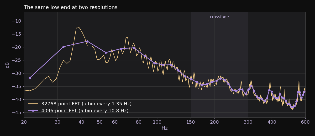 The low end of a loud drum and bass master. The 4096-point curve (purple) has two points between 20 and 40 Hz. The 32768-point curve (gold) has fifteen, and finds a sub peak 5 dB taller than the coarse curve shows.
For mastering, the low end is exactly where precision matters. A sub that sits a few hertz off the kick, or a single bass note ringing louder than the rest, is the kind of thing you open a spectrum to find.
Options
The usual fixes each give something up.
- One long FFT everywhere. A 32768-point FFT has 1.35 Hz bins across the whole spectrum. It also costs more, and the top end doesn’t need it. At 10 kHz you’d be drawing thousands of points per octave to show a curve that’s mostly noise.
- Zero-padding. Padding a short frame out to a longer FFT gives more points, but they’re interpolated between the same 10.8 Hz worth of information. The curve gets smoother without gaining any real frequency resolution.
- Fractional-octave smoothing. Smoothing to 1/3 or 1/6 octave makes the spectrum readable and roughly perceptual, but it erases exactly the narrow peaks we want.
- A constant-Q transform. Bins spaced evenly in log frequency would be ideal on a log axis, but it’s a more expensive and more complicated transform to run over a whole track. I may consider a kernel-based Brown-Puckette Efficient rasterized matrix or Non-Stationary Gabor Frame (NSGF) CQT in a future version of Kouncil.
The key observation is that this is a long-term average. Kouncil’s average spectrum describes the whole track. Time resolution lost by a long FFT in the low frequencies doesn’t matter here at all.
Two FFTs
Kouncil runs two FFTs on each track:
- The ordinary curve is a 4096-point FFT with Hann windows at 50% overlap, averaged over the track.
- A second pass runs a 32768-point FFT the same way, keeping only up to 600 Hz.
A 32768-point frame for every hop of a track is several hundred megabytes at once, so this pass runs one frame at a time instead of the usual vectorized batch.
Below 150 Hz the chart draws the fine curve. Above 300 Hz it draws the coarse one. In between it crossfades linearly from one to the other.
The join sits where the coarse curve stops needing help. By 150 Hz it has about 14 bins an octave, enough to draw a smooth line at a chart’s width, against the two it has between 20 and 40 Hz. By 300 Hz the fine curve has about 220 an octave, more than one per pixel, so going higher would only add points nobody can see.
Density Matching
Broadband sound, like noise or a dense mix, spreads its energy across every bin. With eight times as many bins, each one gets an eighth of the energy. So the long FFT reads broadband content 10·log₁₀(8) ≈ 9 dB lower per bin.
A steady tone behaves differently. It sits in one bin however long the window is, so it reads at the same level in both.
The correction is to add 10·log₁₀(32768 / 4096) back to the fine curve. That turns it into a density, matched to the coarse curve’s scale.
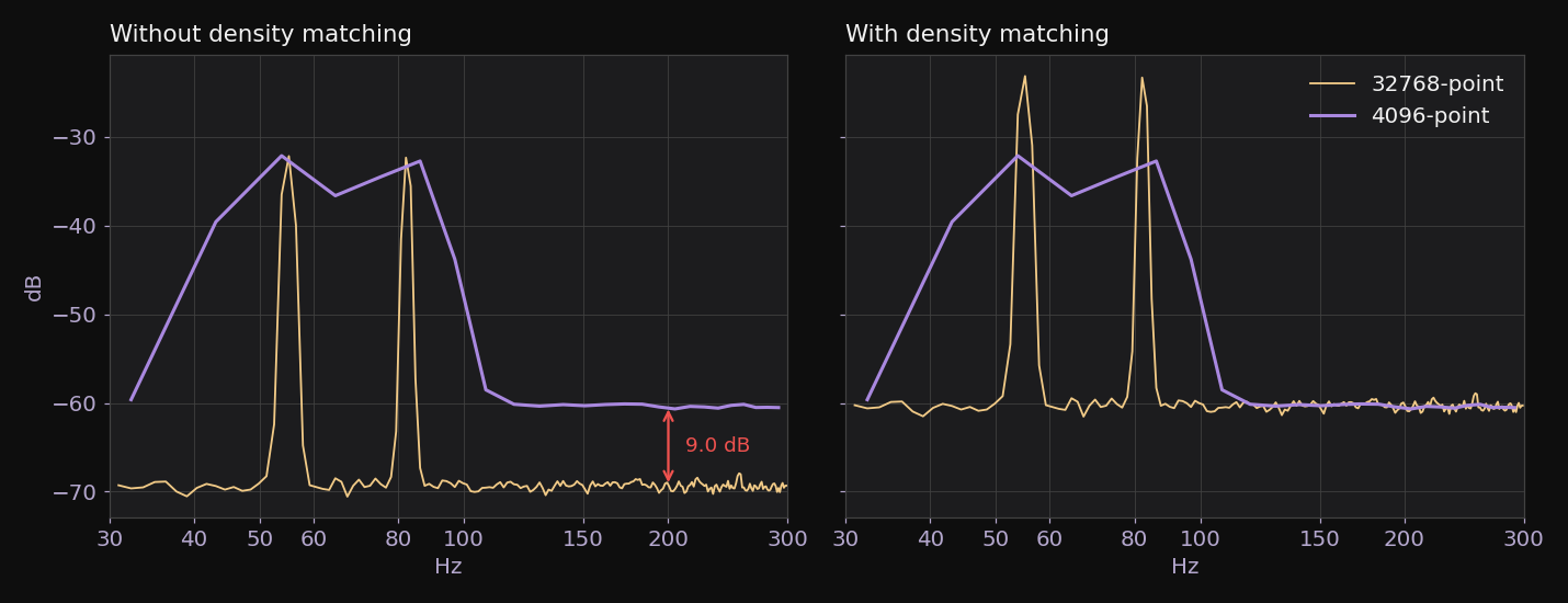 A test signal: white noise plus steady tones at 55 and 82.4 Hz. Without the correction, the fine curve’s noise sits exactly 9 dB under the coarse curve’s. With it, the noise lines up and the tones stand 9 dB taller.
After the correction, broadband content sits at the same level in both curves, so the join is seamless on real music. Tones now stand taller in the fine curve than in the coarse one. That’s intentional. It’s what any analyzer does when you turn its resolution up: the noise floor stays put and the tones resolve out of it.
The figure also shows what the coarse curve does to two notes 27 Hz apart. It draws one wide hump that doesn’t peak at either note.
Other Notes
- Mid/Side. The Mid/Side spectrum goes through the same join, from its own pair of FFTs.
- The left edge. The first bin at or above 20 Hz is a little above it, so the curve would start a few hertz in from the axis. The level at 20 Hz is interpolated and put in front of it.
- Global FFT sharing. Every chart of a spectrum gets its curve from one function that does the join, never recalculated from the raw arrays.
Related Posts
Kouncil: Algorithm Reference
Every analysis algorithm in Kouncil, the mastering analyzer: loudness, dynamics, spectral, perceptual, stereo, codec simulation and render QC.
Kouncil: The Kouncil Members
Kouncil's data-driven music feedback dialogue system.
Inline: Out of Time - Adaptive Soundtrack System Overview
Architecture breakdown of Inline: Out of Time's gameplay-driven adaptive soundtrack system.
Inline: Out of Time - Audio Engine Overview
An overview of the powerful audio engine behind Inline: Out of Time's rich soundscape and audio-driven visuals.